High-Performance Universal GPU Deinterlacing Filter
Author: Kim Bondarenko
Form: Presentation
Level: Advanced
Date: 2026.10.28
What Is Interlaced Video?

A few words about interlaced scanning.
Interlacing and deinterlacing date back to the era of analog television. Interlacing is not simply an obsolete technique that introduces combing artifacts and needs to be corrected. In fact, it is a remarkably effective perceptual technique that significantly reduces the amount of video data transmitted.
Interlacing addresses two requirements at once. In dynamic scenes, viewers perceive motion updated 50 times per second. In static scenes, the image effectively retains the full vertical resolution of a 25 fps video stream, reconstructed from two fields. We will use the 50/25 system as our main example, although the same principles apply to 60/30 and related variants.
This works largely because of the characteristics of CRT displays and the way the human visual system perceives motion and detail. The technique became known as interlaced scanning because alternating fields contain different sets of image lines.
How Does It Work?
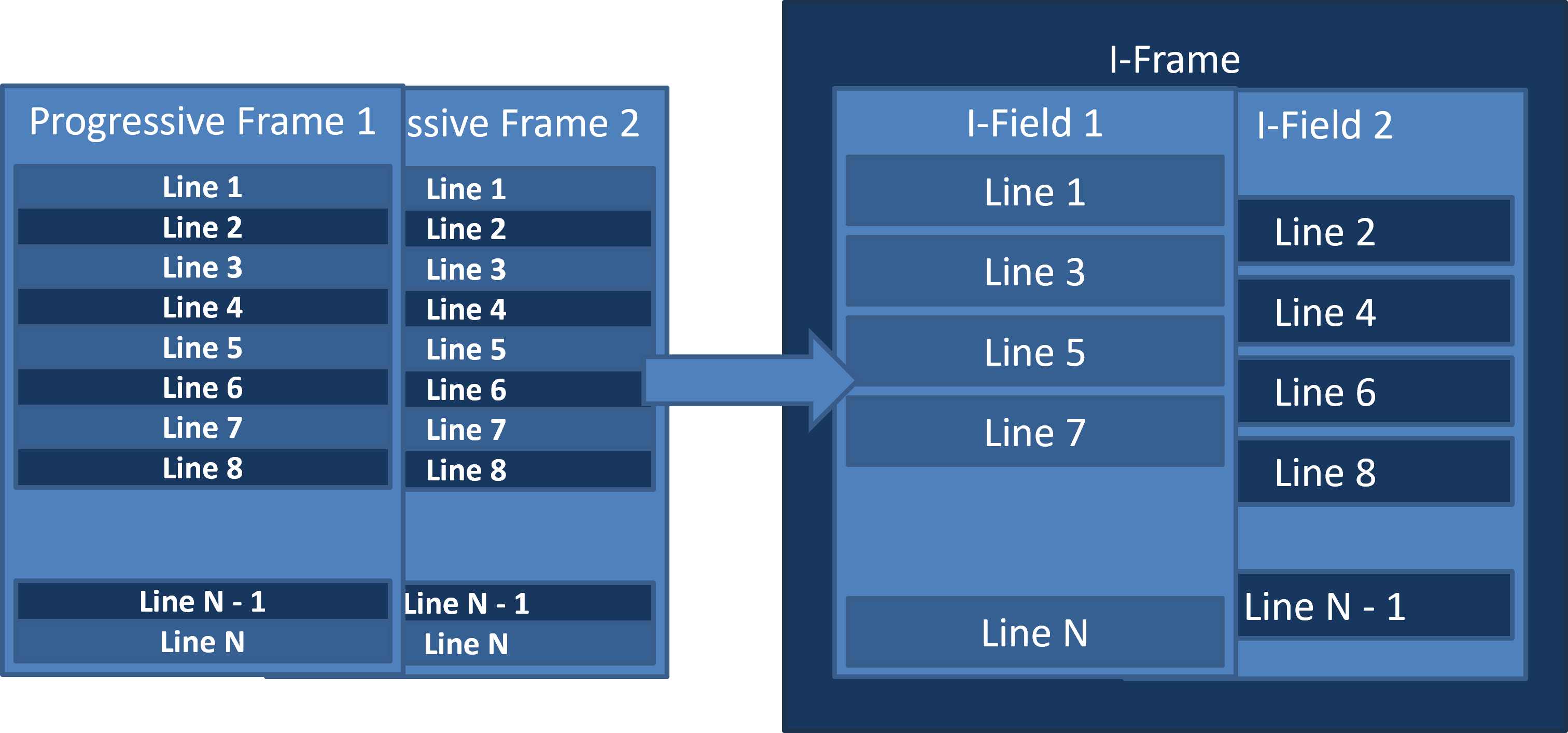
The principle of interlacing is straightforward. One field contains the odd-numbered lines of the image, while the next contains the even-numbered lines captured at a different moment in time. The remaining lines from each source frame are discarded. Together, the two fields form an interlaced frame. Its dimensions match those of the original progressive frame, but the frame rate is halved. As a result, the pixel rate and the bandwidth required for uncompressed video are approximately halved as well.
Interlaced video can be transmitted in different ways. In analog television, the image was transmitted sequentially in fields (half-frames), whose lines alternated on the CRT screen. For example, the PAL/SECAM system used 625 lines per full frame, including vertical blanking intervals, of which 576 lines belonged to the active image. Each field contained 312 or 313 lines, and the parity of the number of lines in a field was used to determine the field's parity.
Digital formats allow interlaced video to be transmitted either as complete frames containing both fields or as separate fields. Unlike analog television, there is no need for electron beam retrace intervals, and the field order is explicitly specified or defined by the format. Typical active image sizes are 576 lines for SD and 1080 lines for Full HD, corresponding to 288 and 540 lines per field, respectively. In practice, this distinction is not particularly relevant to us, since the decoder almost always outputs complete interlaced frames at 25 frames per second.
Interlaced video is conventionally denoted by the lowercase letter i (interlaced), while progressive video usesp (progressive), for example, 1080i50, 1080p50, and 1080p25. The final number indicates the number of fields per second for interlaced video, or frames per second for progressive video.
What Does an Interlaced Frame Look Like?
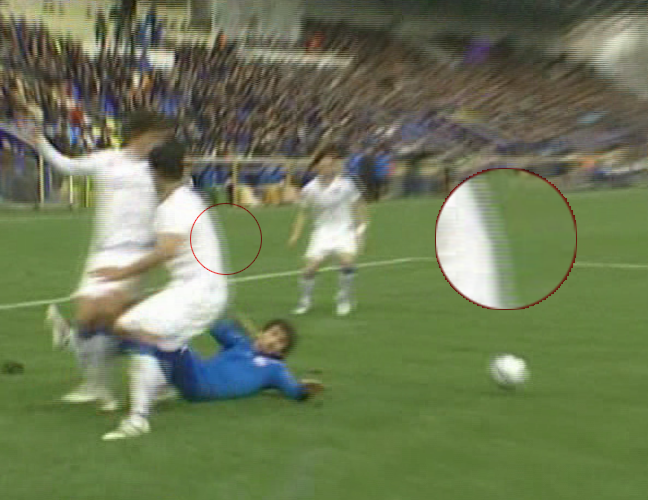
Anyone who has used consumer video players with video content from various sources has probably encountered this kind of video: characteristic combing artifacts and a blurry image.
Many users have wondered why interlacing is needed in digital video at all. The answer is simple: for the same reason as in analog television — to reduce the pixel rate in computationally expensive operations. Video compression has historically been one of the most expensive operations in digital video processing, and to some extent it still is. The same applies to simple per-pixel operations that can be performed directly on interlaced frames, such as adjusting brightness, contrast, and saturation.
What Is a Deinterlacing Filter?
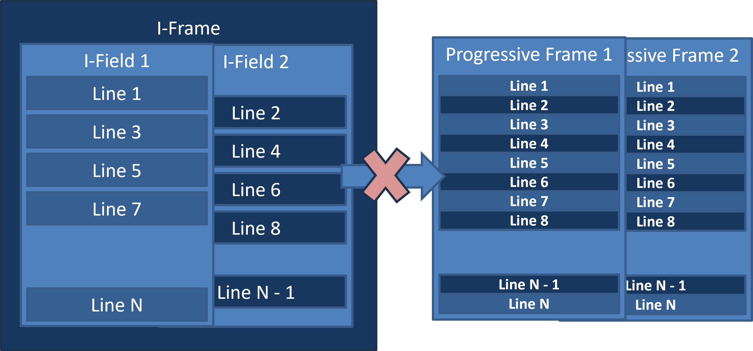
The reverse process is not trivial, since it requires reconstructing data that is missing from the original stream. In practice, however, the task involves much more than simply restoring missing lines.
Sometimes a full-motion 50 fps output is not required. For example, the downstream system may not support this frame rate. Many OTT services process and deliver video at 25 fps only. In this case, the goal is to remove combing artifacts while preserving as much sharpness and spatial detail as possible.
In other cases, a 50 fps output is required, but the source material does not contain 50 distinct frames per second. For example, a 25 fps segment may be inserted into the stream, either as progressive content or as duplicated frames within a 50 fps stream. Depending on the configuration, the filter should output either a 25 fps progressive stream or a 50 fps stream.
Problem Statement
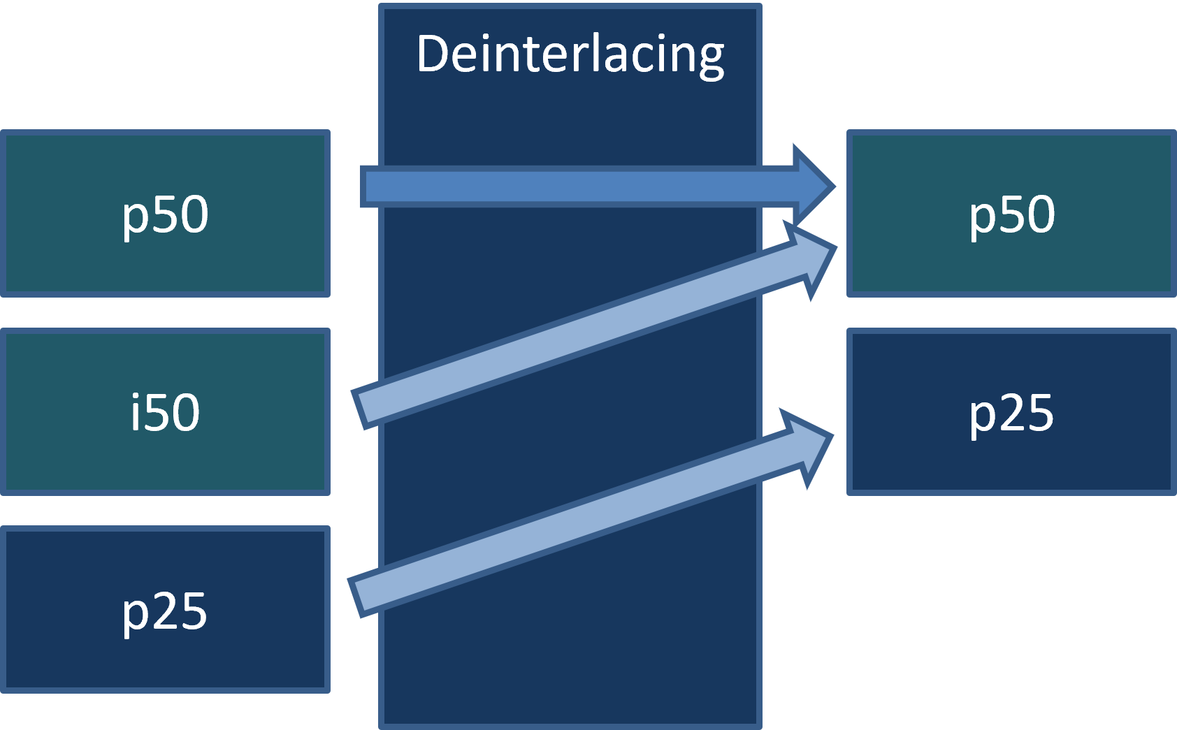
From the transcoder's perspective, the deinterlacing filter is a black box that, depending on its configuration, must output either a progressive p25 stream or a p50 stream, or switch between the two automatically.
At the same time, it must handle different types of input streams and transitions between them in real time. Since frame metadata cannot be relied upon in practice, the filter must have built-in mechanisms for analyzing the actual video content.
When progressive content is detected, the filter must not degrade the image through unnecessary heuristic processing. Instead, the output frame should be assembled directly from the original data, without modifying the pixels.
Stream Types
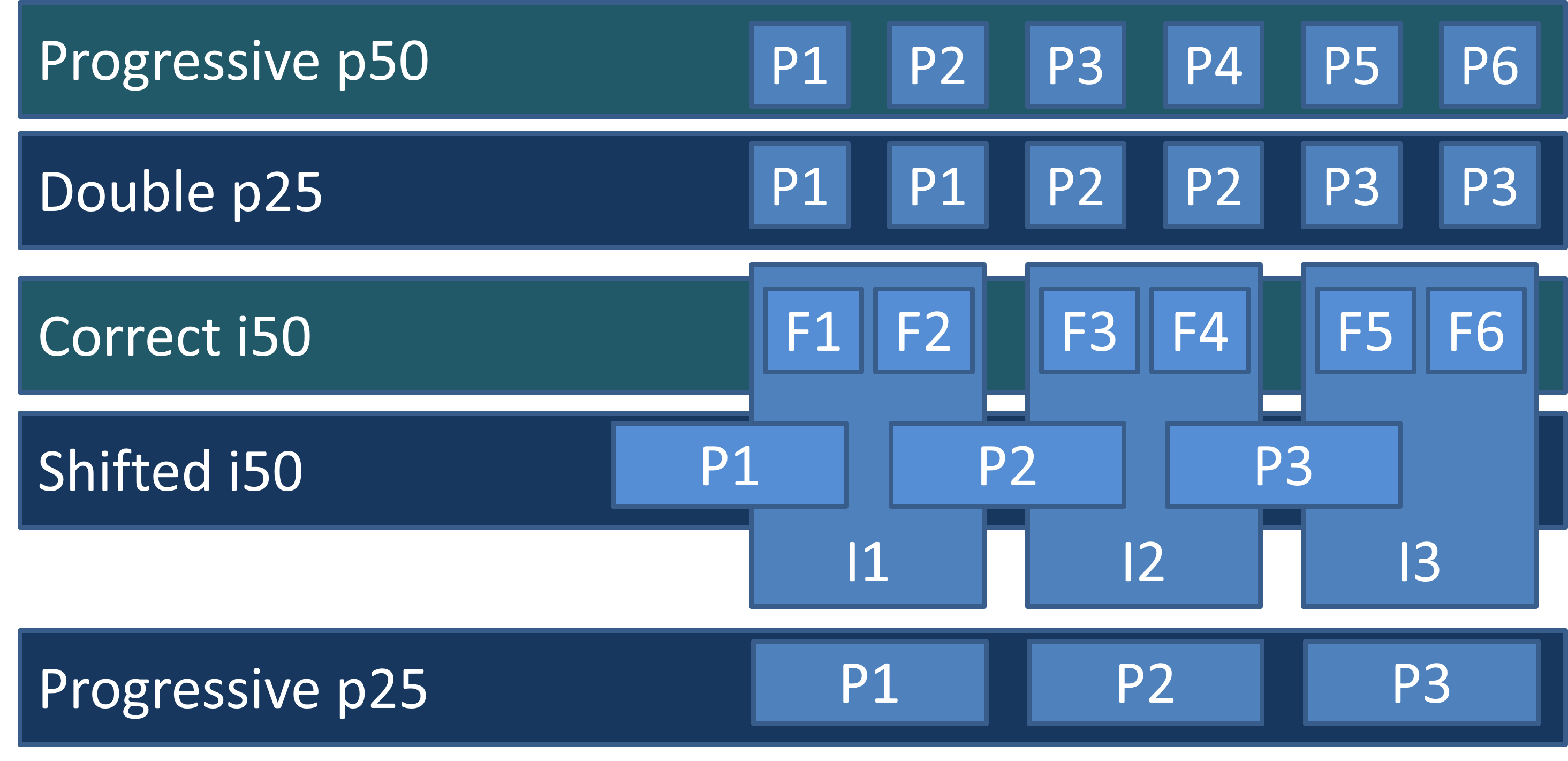
What types of video streams do we encounter in practice? When we started developing this filter, we discovered a real zoo of different cases. After decoding, all we have is the raster image of each frame and its timestamp. In practice, metadata indicating whether the stream is interlaced or progressive cannot be relied upon.
Timestamps allow us to identify streams running at 50 frames per second (the first two rows in the diagram). In these cases, the pixel data does not need to be modified. A proper p50 stream should simply pass through unchanged.
However, what looks like a p50 stream is often actually a sequence of duplicated frame pairs (second row). Depending on its configuration, the deinterlacing filter should detect this case and drop every second frame, producing a proper 25 fps stream.
There is also the classic interlaced i50 stream (third row). The deinterlacing filter must reconstruct a full p50 progressive stream from it.
Another case is a proper progressive p25 stream (last row). Here, the filter should leave the video content completely unchanged.
A more exotic case is so-called shifted interlacing (fourth row). At first glance, the stream looks like ordinary i50 video. However, after reconstructing p50, adjacent frames turn out to be duplicated in pairs, with a temporal offset of one field (half an interlaced frame). This is an unpleasant case, but it can be detected automatically, allowing the correct p25 stream to be restored.
Light green highlights the stream types from which a 50 fps output can be reconstructed. Blue highlights those from which only a 25 fps output can be recovered.
A Short Demonstration
Let's take a short break from the technical details and see the filter in action.
Here is the same video processed by two different filters: the left half shows the result of our algorithm, while the right half shows another reasonably good, fast adaptive filter combining Bob interpolation with Weave reconstruction.
The video has been slowed down by a factor of two to make the difference in motion smoothness easier to see.
The difference is most noticeable in relatively static scenes, where our algorithm reduces high-frequency flickering in high-contrast regions. This is particularly apparent with a stationary camera and in graphical overlays on top of the video.
Detecting Interlaced Video
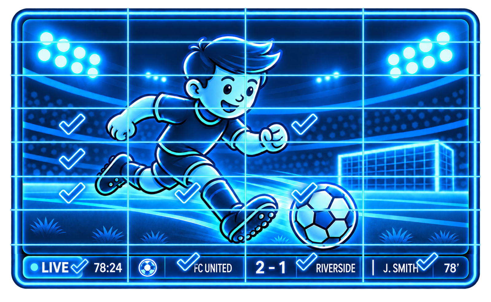
First, let's introduce an interlacing score for each frame — a floating-point value between 0 and 1.
To calculate it, we divide the frame into rectangular blocks and estimate the interlacing level of each block separately. The maximum score across all blocks is used as the interlacing score for the entire frame.
Since interlacing artifacts appear in moving regions, this approach allows us to detect them locally, even when most of the frame is relatively static — for example, when a scrolling ticker is present in a corner of the screen or some object is moving.
For Full HD video, a practical configuration is a grid of 8 columns and 16 rows. This produces horizontally elongated rectangular blocks that are well suited for detecting scrolling text.
If the score exceeds a fixed threshold, the frame is classified as interlaced. Otherwise, it is provisionally considered progressive.
Why provisionally? When evaluating the stream, we should avoid frequent switching between operating modes. Therefore, we take a conservative approach and do not switch to progressive mode immediately after interlacing artifacts disappear. The reverse transition, however, should happen immediately, since leaving combing artifacts unprocessed produces highly visible defects. A reasonable setting is to require 0.5 to 2 seconds without any signs of interlacing before switching to progressive mode.
How to Calculate the Interlacing Score for a Block?
We assume that a normal image has high spatial correlation. This means that neighboring pixels usually differ only slightly.
An interlaced frame combines data from two consecutive fields captured at different moments in time. Even-numbered lines belong to one field, while odd-numbered lines belong to the other. The spatial correlation within each field is therefore generally higher than that of the combined interlaced frame.
For each block, we calculate two measures of spatial pixel differences: f1, treating the image as progressive, and f2, treating it as interlaced. Since we only compare these values, normalization is unnecessary. In practice, f2 represents the combined differences within the two fields. Although each field contains half the pixels of a progressive frame, their combined area is the same, so no division by two is required.
The final score a is calculated as the ratio of f1 to f2. To avoid division by zero, we add a small epsilon value of 0.025f to the denominator. Its exact value is not critical, since the score varies monotonically with the ratio of f1 and f2, and we compare it against a threshold of one.
For a completely static video sequence, the score awill also tend to remain below one, since pixels separated by one intermediate position are generally less correlated than directly adjacent pixels.
Some Code
Shader for calculating the sums of pixel differences
Texture2D<float> tx : register(t0);
RWTexture2D<float2> results : register(u0);

static const int N = 4; // num of 8x8 blocks to process at once

groupshared float2 shared_data[N*8];

[numthreads(8, N, 1)]
void CS(uint3 Gid : SV_GroupID,             // thread group id
        uint3 DTid : SV_DispatchThreadID,   // absolute thread position
        uint3 GTid : SV_GroupThreadID,      // thread position in thread group
        uint GI : SV_GroupIndex)            // thread group scalar index
{
    int2 res = int2(Gid.x*N + GTid.y, Gid.y);  // 8x8 block position

    int iX = GTid.x;    // x-position in block
    int iN = GTid.y;    // block index (0-3)

    int2 ixy0 = res*int2(8, 8);   // block coords

    // load initial data
    float v0 = 0;
    float v1 = tx[ixy0 + int2(iX, 0)];
    float v2 = tx[ixy0 + int2(iX, 1)];

    float2 result = float2(0, 0);
    [unroll] for (int y = 0; y < 8; y++)
    {
        // shift old data and load new data
        v0 = v1;
        v1 = v2;
        v2 = tx[ixy0 + int2(iX, y + 2)];

        // calculation
        result.x += abs(v0 - v1);
        result.y += abs(v0 - v2);
    }

    // store result
    int offset = iN*N;
    GROUP_SUM_VAR(iX, float2, results[res], result, shared_data, 8, offset);
}
Helper for summing values within a ThreadGroup
// shared-memory sync
#define GROUP_SYNC GroupMemoryBarrierWithGroupSync();

// calculates sum of shared-memory array (pow of 2) at first element
#define GROUP_SUMO1(tid, S, shared_array1, N, offset, rest, pitch) \
{   \
    const uint i = (tid); \
    const uint ioffset = (uint)(offset); \
    [unroll] for (uint s = ((N) >> 1); (s > rest); s = (s >> 1)) \
    { \
        [branch] if (i < s) \
        { \
            shared_array1[ioffset + i*pitch] += \
                shared_array1[ioffset + (i + s)*pitch]; \
        } \
        GROUP_SYNC \
    } \
}

// calculates sum of shared-memory array (pow of 2) at dest
#define GROUP_SUMP(tid, S, dest, shared_array, N, offset, pitch) \
{   \
    GROUP_SUMO1(tid, S, shared_array, N, offset, 1, pitch); \
    [branch] if ((tid) == 0) \
        dest = shared_array[offset] + shared_array[offset + pitch]; \
}

// calculates sum of {source} and stores to <dest>
#define GROUP_SUM_VAR(tid, S, dest, source, shared_array, N, offset) \
    shared_array[tid + offset] = source; \
    GROUP_SYNC; \
    GROUP_SUMP(tid, S, dest, shared_array, N, 0, 1);
Here is the code of a compute shader that efficiently calculates both sums of pixel differences, f1 and f2, for an 8×8-pixel block. The result is written to a float2 texture whose resolution is eight times smaller than that of the original image along each axis. The auxiliary code for summing values within a ThreadGroup using GPU shared memory is also included.
Only the Y (luma) plane of the image is analyzed. The UV chroma planes are not involved in the analysis.
The code is written in HLSL. It is vendor-independent and can be easily ported to GLSL.
Calculating Scores for a Rectangular Grid
SComputeConstantsA g : register(b0);

Texture2D<float2> analData : register(t0);
RWStructuredBuffer<float> results: register(u0);

float getFactor(int2 p0, int2 p1)
{
	int npix = 0;
	float sum1 = 0, sum2 = 0;
	for (int y = p0.y; y < p1.y; y++) {
		for (int x = p0.x; x < p1.x; x++) {
			float2 data = analData[int2(x, y)];
			sum1 += data.x;
			sum2 += data.y;
			npix += (8*8);
		}
	}
	if (sum2 < npix*g.plus)
		sum2 = npix*g.plus;

	float factor = sum1/sum2;
	return factor;
}[numthreads(8, 8, 1)]
void CS(uint3 Gid : SV_GroupID, // thread group id
uint3 DTid : SV_DispatchThreadID, // absolute thread position
uint3 GTid : SV_GroupThreadID, // thread position in thread group
uint GI : SV_GroupIndex) // thread group scalar index
{
uint x = DTid.x;
uint y = DTid.y;
if ((x < g.matrix_x) && (y < g.matrix_y))
{
uint2 p0 = uint2(x*g.nsize_x/g.matrix_x,
y*g.nsize_y/g.matrix_y);
uint2 p1 = uint2((x + 1)*g.nsize_x/g.matrix_x,
(y + 1)*g.nsize_y/g.matrix_y);
results[y*g.matrix_x + x] = getFactor(p0, p1);
}
}
Calculating the interlacing score for each rectangular region on the GPU then becomes straightforward. We simply sum the pixel differences from the 8×8 blocks within each region, calculate the ratio of the resulting sums, and write the score to an output buffer. There is little point in performing further processing on the GPU: with a grid of 16 rows and 8 columns, we have only 128 regions. It is easier to transfer this small buffer to the CPU, find the maximum score there, and make the high-level deinterlacing decision.
The Shifted p25 Case
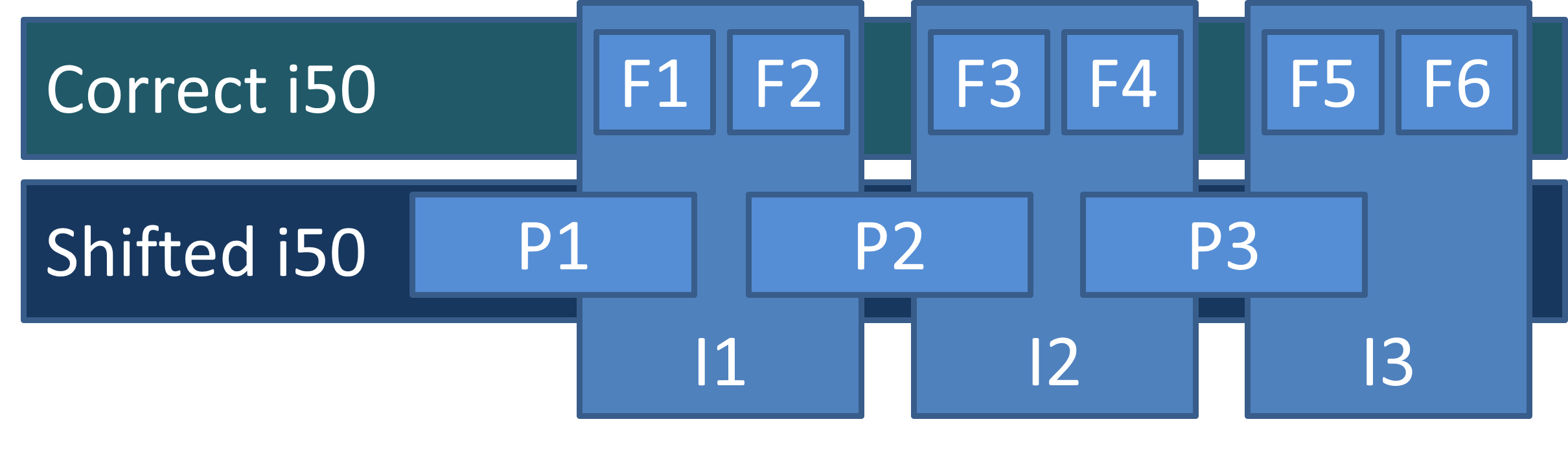
Let's take a closer look at shifted interlacing. This type of stream usually results from peculiarities of the production pipeline: first, 25 fps material is converted to 50 fps by simply duplicating frames. It is then packed back into an interlaced stream, but with a one-field offset. As a result, each interlaced frame contains fields from two adjacent progressive frames of the original video.
The interlacing detector identifies these frames as interlaced. However, if we simply deinterlace the stream and reconstruct p50 video, we find that the expected smoothness is missing: the resulting frames are nearly identical in pairs.
Reconstructing Shifted p25
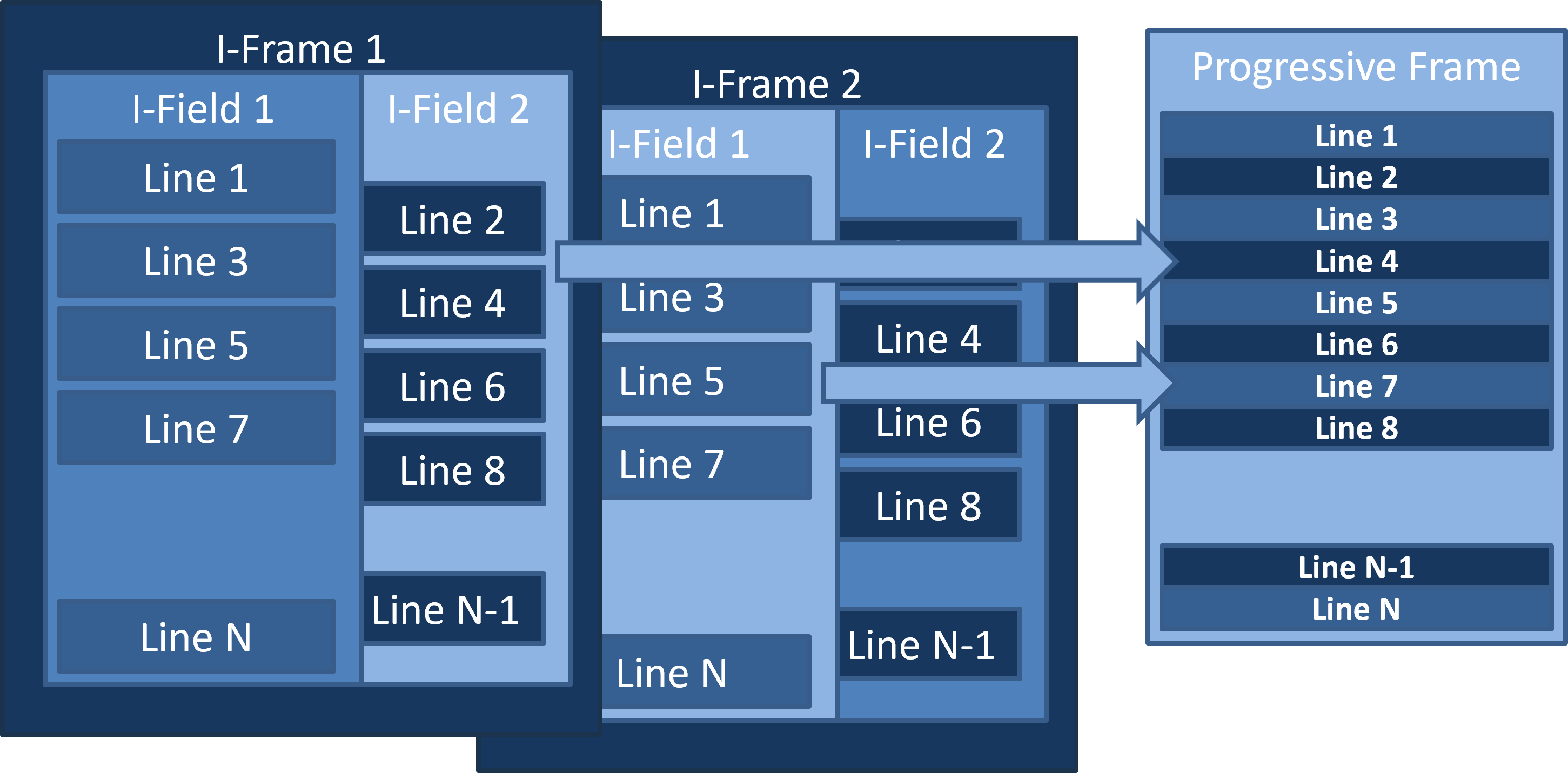
To handle this type of stream correctly, once the interlacing detector reports a positive result, we need to try assembling a candidate frame from the even lines of the current interlaced frame and the odd lines of the next interlaced frame.
If the detector finds no signs of interlacing in the candidate frame, we have identified our case. Instead of applying complex heuristic processing, we simply output the assembled frame as the result.
Full Deinterlacing
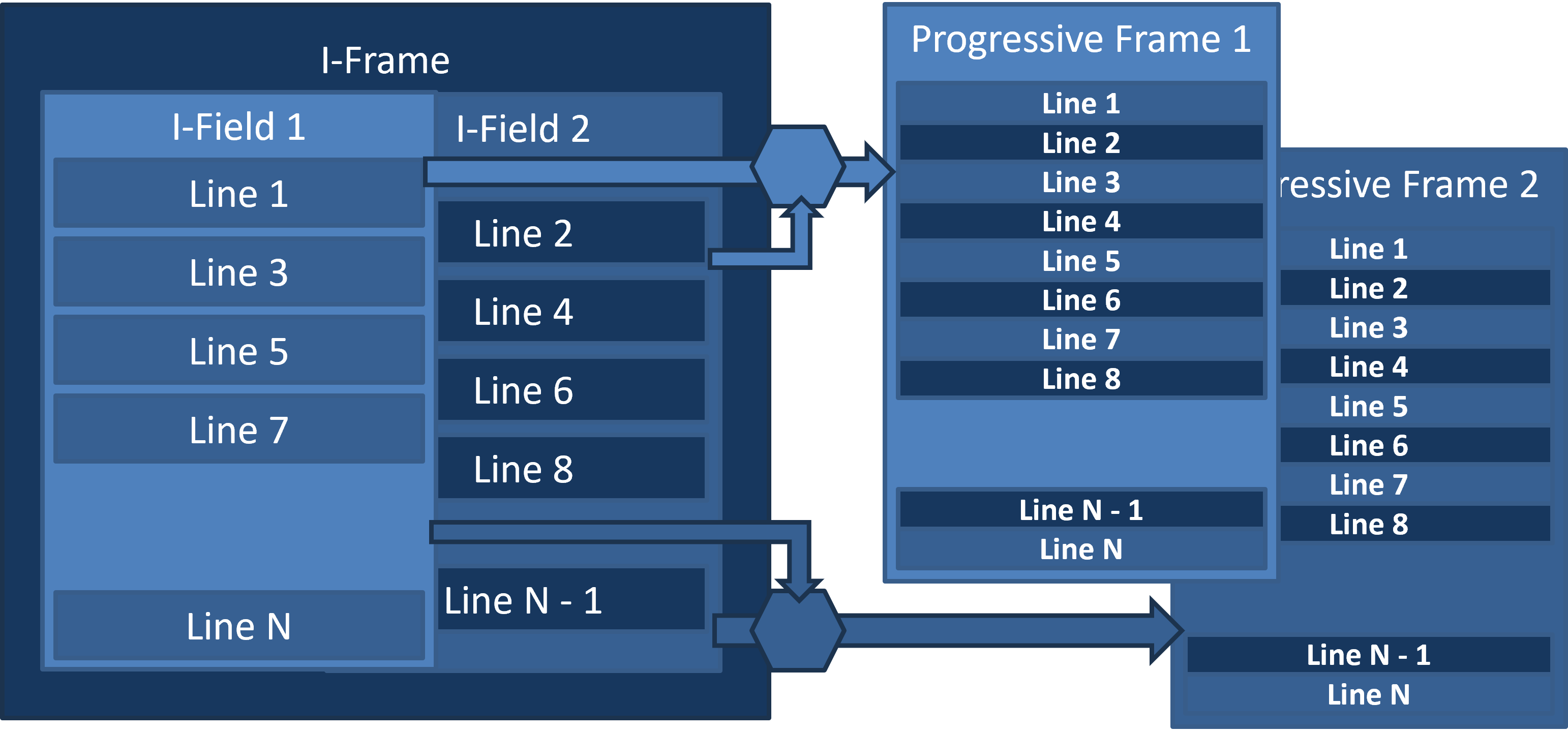
When a frame is unambiguously identified as interlaced, the full deinterlacing procedure must be applied.
The procedure involves reconstructing a progressive frame from two interlaced fields: a primary field and an auxiliary field. The auxiliary field is used to recover spatial details in the image.
In p25 output mode, only one progressive frame is reconstructed from each interlaced frame, using a single reconstruction pass. The first field (odd lines) serves as the primary field, while the second field (even lines) serves as the auxiliary field.
In p50 output mode, two progressive frames are reconstructed from each interlaced frame, conceptually using two passes. The first progressive frame is reconstructed in the same way as in p25 mode. For the second progressive frame, the roles are reversed: the second field becomes the primary field, while the first serves as the auxiliary field. In practice, both passes are combined into a single pass for performance reasons, but this does not affect the mathematical description of the algorithm.
In practice, besides the field order described above (top field first), the reverse order (bottom field first) is also encountered. The field order is a configurable parameter of the filter.
Full Progressive Frame Reconstruction
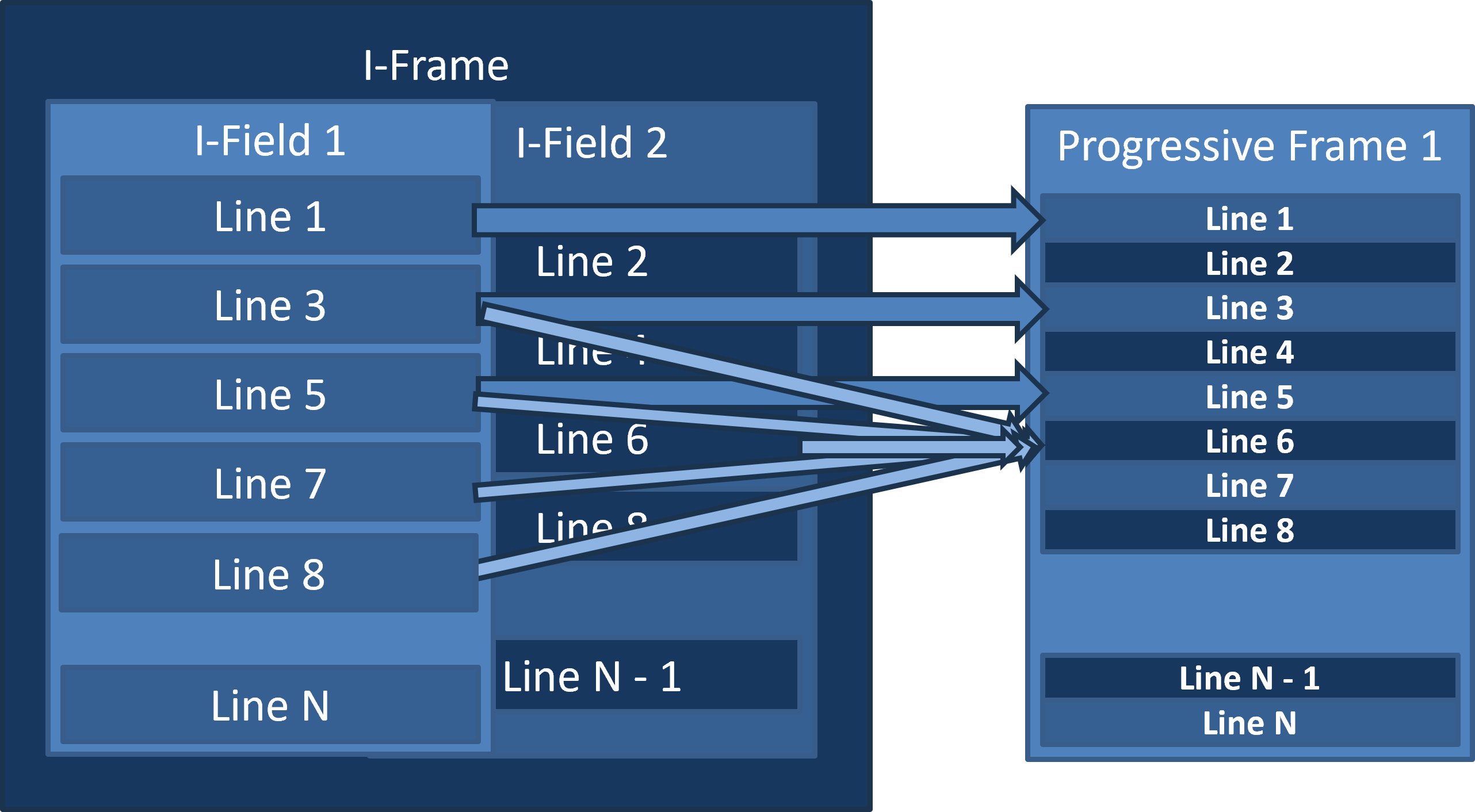
Copying the primary field's lines without modification allows deinterlacing and interlacing filters to be applied sequentially without accumulating computational errors in those lines.
When reconstructing the missing lines, we need to achieve two goals at once. In highly dynamic scenes, we should interpolate between neighboring lines of the primary field, taking the motion in the scene into account. In areas with little motion, we should use data from the auxiliary field to improve the image's vertical resolution, since those samples were captured at vertically offset positions.
How to Kill Two Birds with One Stone?
Now let's dive a little deeper into the mathematics behind the reconstruction process. If you find this section too technical or simply uninteresting, feel free to skip it.
Deinterlacing is performed independently for each field of the interlaced image. Lines belonging to the original field are preserved without modification, while missing lines are reconstructed using motion-adaptive spatiotemporal interpolation.
The algorithm uses three consecutive interlaced frames: the previous frame I₋₁, the current frame I₀, and the next frame I₊₁. Two progressive output frames are generated for each input frame, one for each field. Top Field First (TFF) field order is assumed.
1. Spatial interpolation
Let (x, y) denote the coordinates of the pixel being reconstructed. The initial estimate is the average of the two vertically adjacent pixels in the current frame:
To preserve diagonal edges, we search for the most consistent interpolation direction. Five horizontal offsets are considered: j ∈ {-2, -1, 0, 1, 2}.
For each offset, we calculate the sum of absolute differences between three pairs of pixels on opposite sides of the missing line:
The direction with the lowest matching error is selected:
The spatial prediction is then calculated as the average of the pixels along the selected direction:
2. Temporal prediction
To estimate temporal consistency, pixel values from two frames, A and B, are used. The choice depends on the field being processed: for the first field, A = I₋₁ and B = I₀; for the second field, A = I₀ and B = I₊₁.
The central temporal prediction is calculated as:
The initial allowable deviation is determined by the maximum of three temporal difference measures:
3. Temporal constraints
Additional temporal predictions are calculated for pixels located two lines above and below the pixel being reconstructed:
Here, B_t and F are the upper and lower temporal predictions. For convenience, we also denote the values of the adjacent lines as:
The upper and lower deviation estimates are calculated:
The allowable deviation is then expanded using these estimates:
The final spatiotemporal interpolation result is clamped to an interval around the temporal prediction:
The resulting value is additionally clamped to the [0, 1] range.
4. Motion estimation
To preserve the original detail in static regions, a local motion estimate is calculated using a 5×5-pixel window.
The vertical coordinate of the window center is rounded down to the nearest even line. This ensures that both lines of a pair share the same motion estimation center.
For each pixel in the window, we calculate the maximum difference between the current frame and its temporal neighbors:
The final motion estimate is the average of these differences over the entire window:
5. Adaptive blending
The blending coefficient is derived from the motion estimate using a smoothstep function. Two thresholds are used: a = 0.004 and b = 0.020.
In static regions, the coefficient w approaches zero, preserving the original pixel from the current interlaced frame. When motion is detected, the coefficient increases, giving more weight to spatiotemporal interpolation.
The final reconstructed pixel value is:
Thus, the algorithm combines preservation of original pixel values in static regions (Weave) with directional spatiotemporal interpolation (YADIF) in moving regions.
Optimization
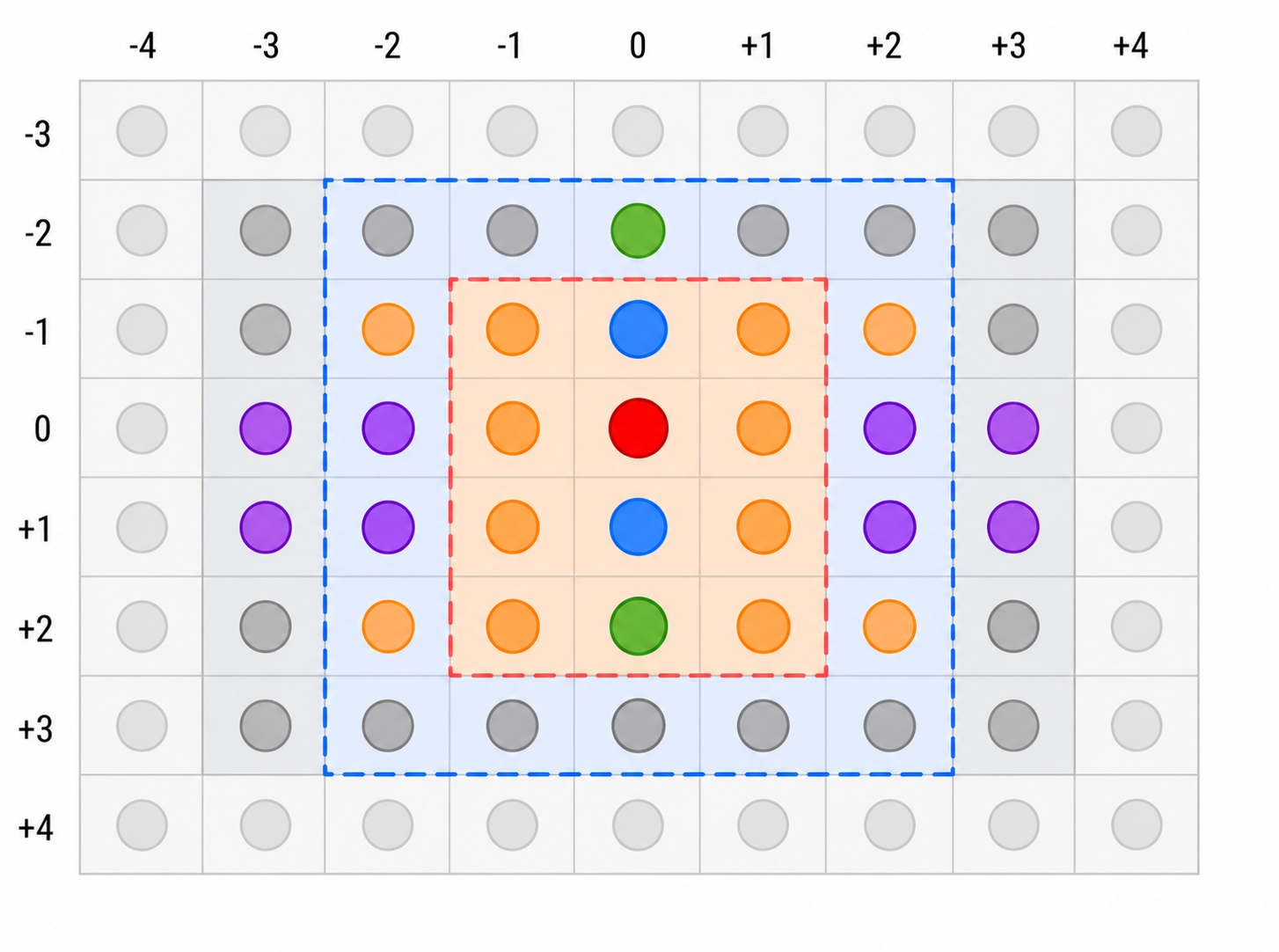
The diagram shows the neighborhood of the pixel being reconstructed, along with the regions used for YADIF spatiotemporal interpolation and motion detection.
- Red — reconstructed pixel.Coordinates (x, y). Its value is calculated using spatiotemporal interpolation and blended with the original value according to the estimated motion.
- Blue — vertical neighbors.Pixels (x, y−1) and (x, y+1) in the current frame. They are used for initial interpolation, directional search, and temporal difference estimation.
- Green — YADIF temporal constraints.Positions (x, y−2) and (x, y+2) in the corresponding pair of frames. They are used to refine the allowable range of the reconstructed value.
- Purple — directional search.Additional pixels used to compare diagonal interpolation directions. The search operates on lines y−1 and y+1 with offsets j = −2, −1, +1, +2.
- Orange — additional pixels.Pixels in the central neighborhood, some of which participate in the YADIF directional search, while others are used for motion estimation.
- Dark gray — surrounding pixels.Pixels in the extended neighborhood. Some are used by the motion detector, depending on whether the reconstructed line is even or odd.
- Light gray — outer region.Pixels outside the main processing region shown in the diagram.
Processing regions
- Red dashed outline.Highlights the central pixel neighborhood for illustration purposes. It does not represent a separate window in the shader.
- Blue dashed outline.Shows the extended neighborhood. The actual motion estimation window is 5×5 pixels and is centered on the nearest even line at or above the reconstructed pixel.
By carefully using compute shaders and shared memory, we can cache much of the overlapping pixel data in fast GPU memory. We can also reconstruct both progressive frames in a single pass, reusing the results of the directional search.
In our experience with similar compute shaders, processing several output pixels per GPU thread works particularly well. This allows each thread group to efficiently process a larger region of the image while reusing data loaded into shared memory.
Main Code — Loading Textures into Shared Memory
Texture2D<S> source0 : register(t0);
Texture2D<S> source1 : register(t1);
Texture2D<S> source2 : register(t2);

SComputeConstantsP g : register(b0);

static const int g_N = 32;  // number of X-threads per group
static const int g_MT = 4;  // number of Y-threads per group
static const int g_MX = 3;  // number of Y-multiplicator

static const int g_M = g_MT*g_MX;

static const int2 lblock2 = int2(g_N, g_M*2);

S readSource(int index, int2 pos)
{
    pos.x = clamp(pos.x, 0, (int) g.size_x - 1);
    pos.y = clamp(pos.y, 0, (int) g.size_y - 1);
    return (index == 0) ? source0[pos] :
            (index == 1) ? source1[pos] : source2[pos];
}

static const int sizeX = g_N + 6;       // group area X-size
static const int sizeY = g_M*2 + 5;     // group area Y-size

static const int pitchX = g_N + 8;
static const int pitchY = sizeY*pitchX;

groupshared S shared_data[3][pitchY];

S readArray(int index, int x, int y)
{
    return shared_data[index][y * pitchX + x];
}
void writeArray(int index, int x, int y, S d)
{
    shared_data[index][y*pitchX + x] = d;
}

S read(int index, int2 pos, int2 posx)
{
    int2 d = pos - posx;
    return readArray(index, d.x, d.y);
}
void preload(int2 delta, int2 posx)
{
[unroll] for (int index = 0; index < 3; index++)
{
S d0 = readSource(index, delta + posx + int2(0, 0));
writeArray(index, delta.x, delta.y, d0);
}
}
void preloadGroup(int2 ithread, int2 posx)
{
const int maxyMT = sizeY/g_MT;
int iy;
for (iy = 0; iy < maxyMT; iy++)
{
int2 pos = int2(ithread.x, (ithread.y + iy*g_MT));
preload(pos, posx);
}
const int extrapix = sizeY*8;
const int extray = (extrapix + g_N - 1)/ (g_N);
const int extrayMT = (extray + g_MT - 1) / g_MT;
for (iy = maxyMT; iy < maxyMT + extrayMT; iy++)
{
int2 pos = int2(ithread.x, ithread.y + iy*g_MT);
[flatten] if (pos.y >= sizeY)
{
// extra field
int i = (pos.y - sizeY)*g_N + pos.x;
pos.x = g_N + (i & 7);
pos.y = (i >> 3);
}
[branch]
if ((pos.x < sizeX) && (pos.y < sizeY))
{
preload(pos, posx);
}
}
GROUP_SYNC
}
This example demonstrates how to cooperatively load a rectangular region from three textures into GPU shared memory. Each thread loads several pixels, distributing the work across the entire ThreadGroup. In addition to the main processing region, we load extra pixels around its edges to support interpolation near the boundaries of the block. The shared-memory row pitch is slightly larger than the actual data width, providing padding for memory layout. Once loading is complete, the threads synchronize to ensure that all data is available before processing begins. This allows neighboring output pixels to reuse the same cached texture data instead of repeatedly accessing the source textures.
S processYADIF(int2 pos, SContext context, int odds)
{
    int2 dx = int2(1, 0); int2 dy = int2(0, 1);

    bool secondField = (odds == 0);
    S p2 = read(secondField ? 0 : 1, pos, context);
    S n2 = read(secondField ? 2 : 0, pos, context);

    S t = (p2 + n2) * 0.5;
    S c = read(0, pos - dy, context);
    S e = read(0, pos + dy, context);

    S diff0 = abs(p2 - n2) * 0.5;
    S diff1 = (abs(read(1, pos - dy, context) - c) +
                abs(read(1, pos + dy, context) - e)
    ) * 0.5;
    S diff2 = (abs(read(2, pos - dy, context) - c) +
                abs(read(2, pos + dy, context) - e)
    ) * 0.5;
    S diff = max(diff0, max(diff1, diff2));

    S spatial = (c + e) * 0.5;
    S score = abs(read(0, pos - dy - dx, context) -
                  read(0, pos + dy - dx, context)) +
              abs(c - e) +
              abs(read(0, pos - dy + dx, context) -
                  read(0, pos + dy + dx, context));

    [unroll] for (int j = -2; j <= 2; j++) {
        if (j == 0) continue;
        int2 shift = int2(j, 0);
        S a0 = read(0, pos - dy + shift - dx, context);
        S a1 = read(0, pos - dy + shift, context);
        S a2 = read(0, pos - dy + shift + dx, context);
        S b0 = read(0, pos + dy - shift - dx, context);
        S b1 = read(0, pos + dy - shift, context);
        S b2 = read(0, pos + dy - shift + dx, context);
        S s = abs(a0 - b0)
                + abs(a1 - b1)
                + abs(a2 - b2);
        compare(s, score, spatial, (a1 + b1) * 0.5);
    }

    S b = (read(secondField ? 0 : 1, pos - 2 * dy, context) +
            read(secondField ? 2 : 0, pos - 2 * dy, context)
    ) * 0.5;
    S f = (read(secondField ? 0 : 1, pos + 2 * dy, context) +
            read(secondField ? 2 : 0, pos + 2 * dy, context)
    ) * 0.5;
    S upper = max(max(t - e, t - c), min(b - c, f - e));
    S lower = min(min(t - e, t - c), max(b - c, f - e));

    diff = max(diff, max(lower, -upper));
    return saturate(clamp(spatial, t - diff, t + diff));
}
struct SContext
{
    int2 posx;
};

S process(int2 pos, SContext context, int odds)
{
    S bob = processYADIF(pos, context, odds);
    S weave = read(0, pos, context);

    int2 base = int2(pos.x, pos.y & ~1);
    S motion = zero;
    [unroll] for (int y = -2; y <= 3; y++) {
        [unroll] for (int x = -2; x <= 2; x++) {
            int2 p = base + int2(x, y);
            S prev = read(1, p, context);
            S cur = read(0, p, context);
            S next = read(2, p, context);
            S d = max(abs(prev - cur), abs(next - cur));
            motion = max(motion, d);
        }
    }
    S weight = smoothstep(0.008, 0.025, motion);
    return lerp(weave, bob, weight);
}

[numthreads(g_N, g_MT, 1)]
void CS(uint3 Gid : SV_GroupID,             // thread group id
        uint3 DTid : SV_DispatchThreadID,   // absolute thread position
        uint3 GTid : SV_GroupThreadID,      // thread position in thread group
        uint GI : SV_GroupIndex)            // thread group scalar index
{

    int2 iblock = Gid.xy*lblock2;
    int2 posx = iblock - int2(3, 2);
    preloadGroup(GTid.xy, posx);

    SContext context; context.posx = posx;
    for (int y = 0; y < g_MX; y++)
    {
        int2 tid = int2(GTid.x, GTid.y + g_MT*y);
        int2 pos = iblock + int2(tid.x, tid.y * 2);
        {
            int2 dy = int2(0, 1);
            int2 pos0 = pos;
            int2 pos1 = pos + dy;
            if (g.odds == 0) {
                pos1 = pos;
                pos0 = pos + dy;
            }
            dest[pos0] = read(0, pos0, context);
            dest[pos1] = process(pos1, context, g.odds);
        }
    }
}
Here is the main part of the reconstruction algorithm. The processYADIF function calculates a missing pixel using three consecutive frames. First, it estimates temporal differences between neighboring frames. It then searches for the most consistent spatial interpolation direction, including diagonal directions, to better preserve slanted edges.
The resulting spatial prediction is constrained by a temporal interval. This prevents the interpolated value from deviating too far from the surrounding pixel values and helps reduce artifacts in moving areas.
The process function combines the YADIF result with the original pixel value using motion-adaptive blending. Motion is estimated from the maximum difference between the current frame and its temporal neighbors within a local window. A smoothstep function converts this estimate into a blending weight: static areas favor Weave, while moving areas favor YADIF interpolation.
Finally, the compute shader processes several pairs of output lines per GPU thread. The original field is copied without modification, while the missing lines are reconstructed. Before processing begins, the ThreadGroup cooperatively loads the required texture region into Shared Memory, allowing neighboring pixels to reuse the cached data.
Conclusion
We started with a seemingly straightforward task: convert interlaced video into progressive frames. In practice, however, a video stream may contain progressive and interlaced content, doubled frames, shifted fields, and transitions between these modes. Applying deinterlacing indiscriminately can degrade perfectly good progressive images.
That is why our filter first analyzes the incoming video and determines which reconstruction strategy is appropriate. Progressive content is preserved, shifted fields can be recombined, and genuinely interlaced frames are reconstructed using motion-adaptive interpolation.
The reconstruction itself combines several ideas: preserving the original field, searching for the best interpolation direction, applying temporal constraints, and blending the result according to the estimated motion. This helps retain fine detail in static areas while reducing combing artifacts and flickering in moving scenes.
Finally, performance matters just as much as image quality. Compute shaders, shared memory, cooperative texture loading, and processing multiple pixels per GPU thread allow us to reuse data and reduce memory traffic. These optimizations make the approach suitable for real-time video processing.